
Neural nets (almost) from scratch
Published:
One thing that every data scienctist knows is how to deploy a neural net of its advanced versions using one of the big python libraries like tensorflow or pytorch. So why go through the pain of writing the model from (almost) scratch?
Designing a ML model for a given dataset requires the programmer to go through certain steps, first to preprocess the data aand the second is tuning the parameters of the model. This article will delve into the second part and explain how learning the workings of a ML model might help us understand parameter tuning. I’ll begin with a basic neural net with a few hidden layers.
A basic neural net can be visualized as:
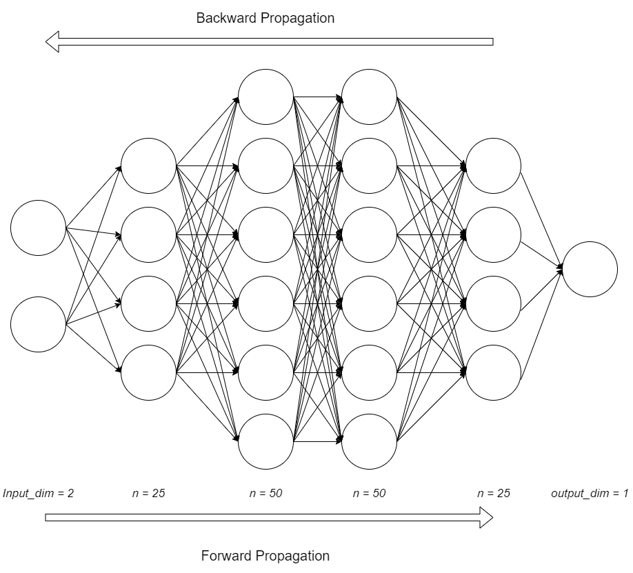
This is the basic model architecture that will be followed in this post. As can be seen, a two dimensional input will be inputted to the model, and the model solves a classification problem, hence only a single input will decide if the input belongs to a community or not.
The basics
Forward propagation in a neural net is similar to a linear regression. This means that for each unit in each layer the weights of the regression equation have to be stored, to enable easy access. The parameters are stored in a navigable data structure (a list in this case, for simplicity) labelled param_cache, similarly the output values of the cells are stored in a seperate memory cache named memory (data structure same as that used in param_cache).
Defining the model architecture in python
A python list stores the characteristics of each layer, using dictionaries to store variables.
An additional variable mentioned here is the activation function. Rest assured, further sections will cover these functions. For now we move towards layer initiation. The input_dim variable specifies the length of input array, and a similar case is true ffor the output_dim. By intuition, the output of one layer will be the input of next layer, a symmetry which can easily be observed.
The above snippet initiates the memory cache which will store the variables for each layer, and as evident from the code initially the regression weights are initiated to random values to break symmetry, else the model will become a single linear regression without the ability to capture information.
Activation functions
Activation functions are applied on functions often to bonud the output values within certain ranges, and to introcude non-linearity into the model. The functions implemented in the library are the ‘ReLU’ and ‘sigmoid’. ReLU activation has often proven to be appropriate for hidden layers, since it allows selective transmission of information across the model. The final activation function can be ‘sigmoid’ or ‘linear’ based on whether the problem solves ‘classification’ or ‘regression’ respectively.
Forward propagation
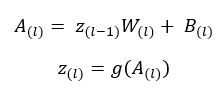
I’ll introduce a few variable names here to be used for the rest of the post. Referring the above image, z is the layer input array, A is the inactivated layer output, W are the layer weights, B is the layer bias value (defined similarly to the constant term in linear regressions) and g() is the activation function. The subscript of the variables denote the layer index.
The above snippet is the forward propagation through a single layer. full_forward_prop.py is a complete loop of forward propagation for one iteration, and it stores the layer outputs in the memory as it goes through the layers.
Backward propagation
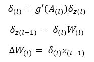
The back propagation of error in neural nets optimizes the parameter values of each layers based on the penalty incurred after one iteration of forward propagation. The derivatives are calculated simply by chaining derivatives of the output values between layers.
Above snippet is a complete loop of backward propagation accross the model. The first penalty in the model is introduced at the last output layer, when the error is calculated by measuring the distance between the output and the target.
Learning phase
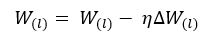
Once change required in the parameter is calculated, the parameters are updated according to the equation above, where “neta” is the learning rate chosen by the user.
Wrapping it all up!
Finally all functions are packed up in sequence as: The above snippet outputs the model parameters trained on a input dataset along with the true output values. Finally, the parameter cache returned by the above function is run on the test input data, which generates the output for the test data inputs.
Scoring and accuracy
The scoring algorithms above are quite basic, and can work well for small or medium datasets. Test example for this library was implemented on the scikit make_moons data, which generates 1000 points to be classfied into two categories. This model with the architecture mentioned earlier gave an accuracy of 85%, a value which can be imrpoved with optimizers.
Access the main library and the test exmaple here
Future Scope
I was inspired to write the blog after going through Andrew Ng’s lecture series and especially the article on neural nets posted by Piotr Skalski on medium. After studying about neural nets, I realized the importance of taking a deep dive into AI models before implementing the models using larger python libraries, and Piotr’s article provided me a methodology to understand and implement the models from scratch. It will be my aim to implement every model I learn about similarly, along with the usage of optimizers wherever required.